Arrays of counts at each transcript position
Many next-generation sequencing assays capture interesting features of biology with nucleotide precision. It is convenient to represent data from such an assay as an array of numbers, each position in the array corresponding to a position in some region of interest, like a transcript.
This tutorial shows how to obtain such arrays (as
numpy arrays), which can be subsequently mainpulated
by downstream tools. In this example, we’ll extract arrays of the number of
ribosomal P-sites at each position in a transcript from
ribosome profiling data. However, with appropriate
alignment mapping rules, the code below could
fetch arrays of virtually any biological feature captured in a set of read
alignments.
In the examples below, we use the Demo dataset.
Contents:
Working with vectors of counts interactively
Retrieving the arrays
To count read alignments along a transcript, we need:
An annotation of transcript models. In this case, a BED file, which we’ll read using a
BED_Reader.A high-throughput sequencing dataset. In this case, read alignments in a BAM file, imported into a
BAMGenomeArray.
First read the transcripts:
# import plastid
# data structure for mapping read alignments to genomic positions
>>> from plastid import BAMGenomeArray, FivePrimeMapFactory, \
                        BED_Reader, Transcript


# load the transcript annotations from the BED file.
# BED_Reader returns an iterator, so here we convert it to a list.
>>> transcripts = list(BED_Reader("merlin_orfs.bed",return_type=Transcript))
Then, load the ribosome profiling data. We’ll map read alignments to their corresponding P-sites, estimating the P-site to be 14 nucleotides from the 5’ end:
# load ribosome profiling data
>>> alignments = BAMGenomeArray("SRR609197_riboprofile_5hr_rep1.bam")

# set P-site mapping as 14 nucleotides from 5' end
>>> alignments.set_mapping(FivePrimeMapFactory(offset=14))
Now, we’re ready to count. The method
get_counts(), returns
a numpy array of counts at each position in the
transcript, from the transcript’s 5’ end to its 3’ end (for reverse-strand
features, counts are reversed relative to genomic coordinates), accounting for
splicing of exons:
# create a list to hold the vectors
>>> count_vectors = []

# get counts for each transcript
>>> for transcript in transcripts:
>>>     count_vectors.append(transcript.get_counts(alignments))
Manipulating arrays
Now that we have a list of numpy arrays, we can
manipulate them like any other numpy array:
# we'll take transcript 53 as an example- it has lots of reads
# check the lengths of the first transcript and its vector.
# they should be identical
>>> my_transcript = transcripts[53]
>>> my_vector = count_vectors[53]

# lengths should match
>>> my_transcript.length, len(my_vector)
(1571, 1571)

# get total counts over entire array
>>> my_vector.sum()
7444.0

# look at counts at positions 200-250 of the array
>>> my_vector[200:250]
array([   7.,   25.,   18.,   13.,    5.,    1.,   11.,    3.,    0.,
          1.,   25.,   11.,   29.,   27.,   18.,    3.,   16.,   20.,
         10.,    0.,    4.,   20.,   10.,    2.,    3.,   19.,    4.,
          9.,    1.,   15.,    5.,    3.,   11.,    8.,   13.,   15.,
          4.,  121.,    3.,    6.,   45.,    3.,    4.,   39.,   14.,
          3.,    9.,    7.,    8.,   24.])
Because the vector is a numpy array, it can be
manipulated using the tools in numpy, SciPy, or matplotlib:
>>> import numpy

# mean & variance in coverage
>>> my_vector.mean(), my_vector.var()
(4.7383831954169322, 49.177260021207104)

# location of highest peak
>>> my_vector.argmax()
237

# take cumulative sum
>>> my_vector.cumsum()
array([    0.,     0.,     0., ...,  7444.,  7444.,  7444.])

# 30-codon sliding window average
>>> window = numpy.ones(90).astype(float)/90.0
>>> sliding_window_avg = numpy.convolve(my_vector,window,mode="valid")


# plot
>>> import matplotlib.pyplot as plt

>>> plt.plot(my_vector,label="%s counts" % my_transcript.get_name())
>>> plt.plot(sliding_window_avg,label="30 codon average")
>>> plt.xlabel("Position in transcript (5' to 3')")
>>> plt.ylabel("Ribosome counts")

>>> # add outlines at start & stop codons
>>> plt.axvline(my_transcript.cds_start,color="#999999",dashes=[3,2],zorder=-1)
>>> plt.axvline(my_transcript.cds_end,color="#999999",dashes=[3,2],zorder=-1)

>>> plt.legend()
>>> plt.show()
This makes the following figure:
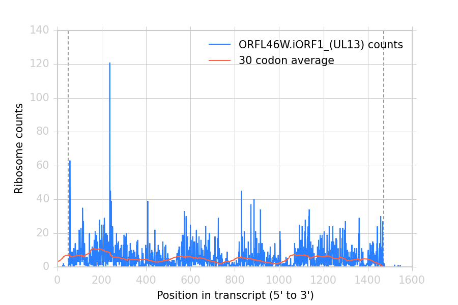
Ribosome density at each position in a sample transcript. Dashed vertical lines: start and stop codons.
Using the get_count_vectors script
The analysis above is implemented by the command-line script get_count_vectors,
which fetches an array for each feature in an annotation file, and saves it
as a file named for that feature.
As above, we’ll use ribosome profiling data and map read alignments to their
estimated P-sites, 14 nucleotides from their 5’ ends. The arguments
--fiveprime --offset 14 handle this. The script may be executed from the
terminal:
$ get_count_vectors --annotation_files merlin_orfs.bed \
                    --annotation_format BED \
                    --count_files SRR609197_riboprofile_5hr_rep1.bam \
                    --fiveprime \
                    --offset 14 \
                    folder_of_arrays
Each output file will be saved in folder_of_arrays and named for the transcript_ID or ID attribute of the corresponding genomic feature:
$ ls folder_of_arrays
ORFL100C.txt               ORFL169C.txt                 ORFL237C.txt                    ORFL308C_(UL139).txt         ORFL85C_(UL30).txt
ORFL101C.iORF1_(UL36).txt  ORFL16C.iORF1.txt            ORFL238W.iORF1.txt              ORFL309C.txt                 ORFL86W.txt
ORFL101C.txt               ORFL16C.txt                  ORFL238W.txt                    ORFL30W.txt                  ORFL87W.txt
ORFL102C.iORF1.txt         ORFL170C.txt                 ORFL239C.txt                    ORFL310W.txt                 ORFL88C.iORF1.txt
ORFL102C_(UL38).txt        ORFL171W.txt                 ORFL23W_(RL12).txt              ORFL311W.txt                 ORFL88C_(UL30A).txt
ORFL103C_(vMIA).txt        ORFL172W.txt                 ORFL240C.txt                    ORFL312C.txt                 ORFL89C.txt
ORFL104C_(UL37).txt        ORFL173W.txt                 ORFL241C_(UL103).txt            ORFL313C_(UL138).txt         ORFL8C.txt
ORFL105C_(UL40).txt        ORFL174C.iORF2.txt           ORFL242W.txt                    ORFL314C.iORF1.txt           ORFL90C.txt
(rest of output omitted)
The output can be loaded into numpy arrays using
numpy.loadtxt():
>>> import numpy

>>> my_reloaded_vector = numpy.loadtxt("folder_of_arrays/ORFL46W.iORF1_(UL13).txt")
>>> my_reloaded_vector[200:250]
array([   7.,   25.,   18.,   13.,    5.,    1.,   10.,    3.,    0.,
          1.,   24.,    9.,   27.,   27.,   18.,    3.,   16.,   20.,
         10.,    0.,    4.,   20.,   10.,    2.,    3.,   19.,    4.,
          9.,    1.,   15.,    5.,    3.,   11.,    8.,   13.,   14.,
          4.,  119.,    3.,    6.,   45.,    3.,    4.,   39.,   14.,
          3.,    9.,    7.,    8.,   24.])
Masking unwanted regions
get_count_vectors can optionally take a mask file to exclude
problematic regions from analysis. Interactively, regions can be masked using
add_masks() and masked arrays
obtained using get_masked_counts().
In these cases, vectors are returned as numpy.ma.MaskedArray objects,
and positions annotated in the mask file are given the value
numpy.NaN instead of their numerical values.
See Excluding (masking) regions of the genome for details on using masks and creating mask
files using the crossmap script.
See also
plastid.readers, readers for various file formats used in genomics
plastid.genomics.genome_array, GenomeArray classes for BigWig, wiggle, bedGraph and bowtie files
SegmentChainandTranscriptfor full documentation of what these objects can do