Performing metagene analyses

Definition

A metagene analysis is an average of quantitative data over one or more genomic regions (often genes or transcripts) aligned at some internal feature. For example, a metagene profile could be built around:

• the average of ribosome density surrounding the start codons of all transcripts in a ribosome profiling dataset

• an average phylogenetic conservation score surounding the 5’ splice site of the first introns of all transcripts

Often, this sort of analysis reveals patterns across regions that may not be obvious when looking at any individual region.

Scope of this tutorial

In this tutorial, we:

• Use the metagene script to perform a metagene analysis of ribosome density surrounding start codons in a ribosome profiling dataset

• Discuss how to write functions to perform custom metagene analyses surrounding arbitary features of interest. As an example, we make a metagene average of ribosome density surrounding the highest peak of ribosome density in coding regions.

This tutorial uses the Demo dataset we have prepared.

Computation

A metagene average is computed by:

1. Fetching vectors of quantitative data – in this example, ribosome-protected footprints – surrounding each occurrence of the feature of interset – in this case, a start codon – in each region:

   

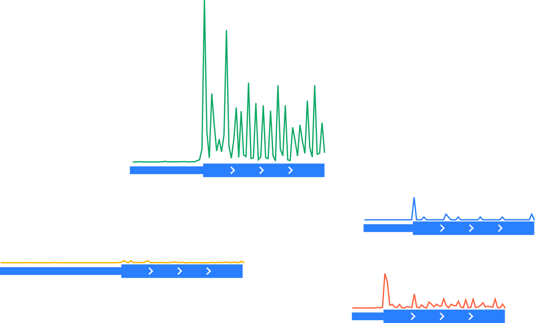
   Unnormalized vectors of ribosome-protected footprints, shown above corresponding transcript models. Thick boxes: coding regions. Thin boxes: 5’ UTRs.

2. Normalizing each vector to the same scale by dividing by the total number of counts in a normalization window (here, the last 30 nucleotides of the portion of coding region shown):

   

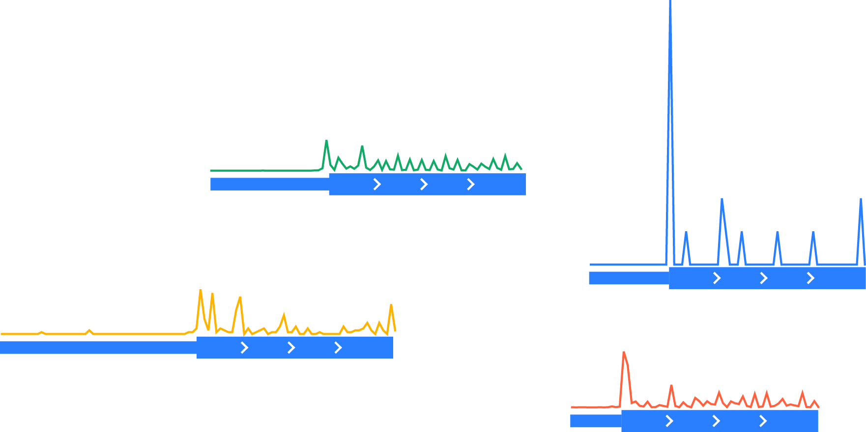
3. Aligning each vector at the feature of interest (the start codon)

4. Taking an average (e.g. a median, mean, or percentile) over all of the normalized vectors at each aligned nucleotide position. Typically, we use the median:

   

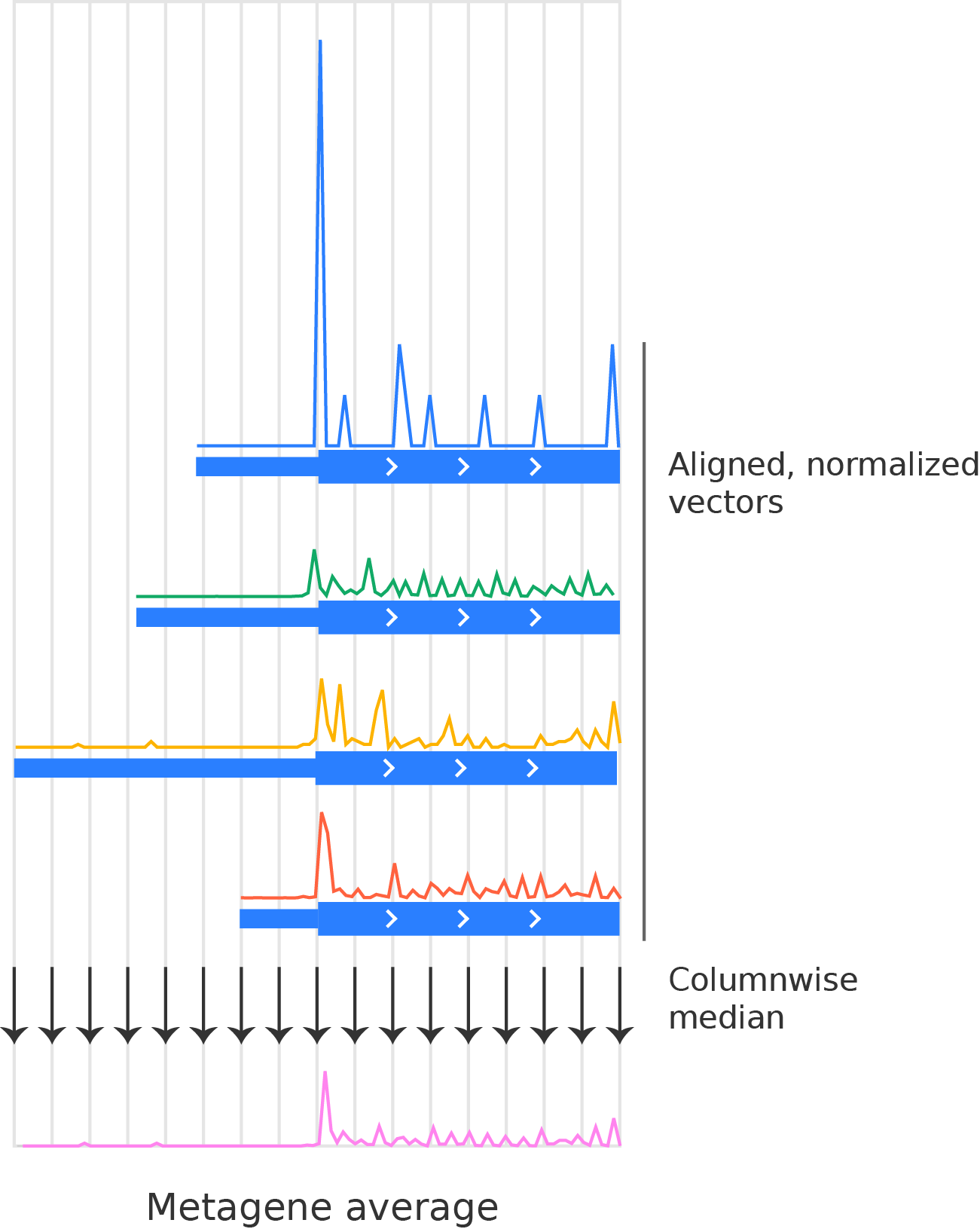
   Final metagene average over the four transcripts shown above.

Using the metagene script

When called from the command-line, metagene divides the analysis into two subprograms:

• The generate subprogram processes a genome annotation into a set of aligned windows surrounding a feature of interest (e.g. a start codon)

• The count subprogram takes the revised annotation from generate and a dataset of read alignments or other quantitative data, and produces the metagene average

For convenience, a chart subprogram is also provided to plot the outcome of one or more runs of the count subprogram.

The generate subprogram

The first step in a metagene analysis is to examine all of the regions of interest – in this example, transcripts – in a genome annotation, detect an interesting sub-feature – here, a start codon – and build a sub-window within the transcript that surrounds the sub-feature. To do so, the metagene generate subprogram performs the following steps:

1. Group transcripts by gene, so each start codon is only counted once.

2. If a gene has multiple start codons, exclude that gene.

   If a gene has a single start codon, then find the maximal spanning window of the gene, defined as the largest possible window surrounding the start codon in which all transcripts from that gene map to identical genomic positions. This prevents any positional ambiguity from entering the average:

   

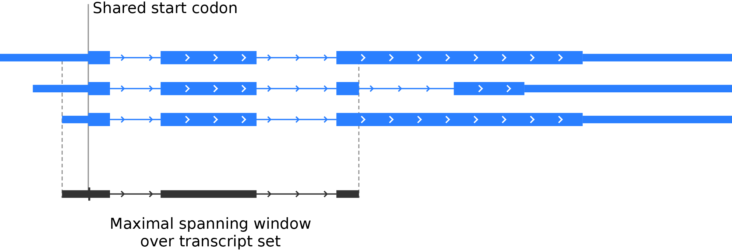
3. Once a maximal spanning window is defined for a gene, determine the location of the start codon relative to the window, so that the maximal spanning windows for all genes may be aligned at the start codon during the count step.

4. Save the maximal spanning windows to a BED file for inspection in a genome browser or other analysis pipeline, and to a text file (called an ROI file) for use in the count subprogram.

The generate program only needs to be run once per landmark of interest (i.e. once for stop codons, once for start codons), and only needs to be re-run if the genome annotation changes (e.g. due to revisions, additions, or deletions of gene/transcript models).

We will run the generate program using the following arguments:

• merlin_cds_start : name all output files with the prefix merlin_cds_start

• --landmark cds_start : calculate a metagene average surrounding start codons

• --annotation_files merlin_orfs.gtf : use transcript models from this annotation file

• --downstream 200 : include up to 200 nucleotides downstream of the start codon in the average

The program is called from the terminal:

$ metagene generate merlin_cds_start --landmark cds_start \
                                     --annotation_files merlin_orfs.gtf \
                                     --downstream 200

For a detailed description of these and other command-line arguments, see the metagene script documentation

The count subprogram

Once generate has made an ROI file, metagene’s count subprogram can be used to tabulate metagene averages. Specifically, count performs the following steps:

1. For each maximal spanning window in the ROI file:

   1. fetch a vector of counts at each position from the sample dataset (in this case, ribosome profiling alignments).

   2. If the vector of counts has a sufficient number of alignments within a user-specified normalization region, include it. Otherwise, exclude the vector.

   3. Normalize the vector by the total number of counts in the normalization region.

2. Construct a metagene average by taking the median over all normalized vectors at each position, excluding any vectors that happen not cover that position (e.g. because the maximal spanning window for that gene was too small).

3. For each position, save the metagene average and the number of genes included in the average to a tab-delimited text file.

To call the count program, type into a terminal window. In this example, the parameters --fiveprime --offset 14 specify our mapping rule for the P-site offset, estimating the offset as 14 nucleotides from the 5’ end of each read alignment. The parameter --normalize_over 30 200 indicates that each vector should be normalized to the total number of counts it contains in the region from 30 to 200 nucleotides downstream of the start codon. The parameter --min_counts 50 ensures that we’re only including genes that have at least 50 counts in the region we’re normalizing over:

$ metagene count merlin_cds_start_rois.txt SRR609197_riboprofile \
                 --count_files SRR609197_riboprofile_5hr_rep1.bam \
                 --fiveprime --offset 14 --normalize_over 30 200 \
                 --min_counts 50 --cmap Blues --title "Metagene demo"

A number of files are created and may be used for further processing. In our example, SRR609197_riboprofile_metagene_profile.txt contains the final, reduced data. This file contains three columns:

1. x: an X-coordinate indicating the distance in nucleotides from the start codon

2. metagene_profile: the value of the metagene average at x

3. regions_counted: the number of regions included in the average at x

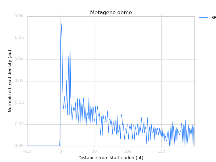
The chart subprogram

For convenience, a chart subprogram is included. It can plot multiple metagene profiles (each from a run of the count subprogram) in a single plot:

$ metagene chart SRR609197_riboprofile_cds_start.png \
                 SRR609197_riboprofile_metagene_profile.txt \
                 --landmark "start codon" \
                 --title "Metagene demo"

This produces the image:

Metagene profile surrounding start codon.

Beyond start and stop codons: defining your own window functions

Metagene averages can be useful for other questions, types of regions, and experimental data. For this reason, metagene offers tools to create maximal spanning windows surrounding any feature of interest.

Window functions

To make maximal spanning windows around a feature, metagene requires a window function. The window function must identify and build a window around the feature of interest (e.g. a start codon) in each individual region examined (for example, each transcript).

metagene comes with two window functions:

• window_cds_start(), for defining windows surrounding start codons

• window_cds_stop(), for defining windows surrounding stop codons

Once you have defined a window function, plastid.bin.metagene.group_regions_make_windows() can use it to generate maximal spanning windows.

Parameters

Window functions must take the following parameters, in order:

roiSegmentChain

Input ROI for which a window will be generated. If “gene_id” is defined in roi.attr, then all roi`s sharing the same `”gene_id” will be used to generate a single maximal spanning window covering all of them.

flank_upstreamint

Nucleotide length upstream of the feature of interest to include in the maximal spanning window, if roi has such a feature

flank_downstreamint

Nucleotide length downstream of the feature of interest to include in the maximal spanning window, if roi has such a feature

ref_deltaint, optional

Offset in nucleotides from the feature of interest to the reference point at which all maximal spanning window count vectors will be aligned when the metagene average is calculated. If 0, the feature of interest is the reference point. (Default: 0)

Return values

Window functions must return the following values, in order:

SegmentChain

Window surrounding feature of interest if roi has such a feature. Otherwise, return a zero-length SegmentChain. plastid.bin.metagene.do_generate() will use these to generate maximal spanning windows.

int

offset to align window with all other windows, calculated as max(0,flank_upstream - distance to reference point from 5' end of window), or numpy.nan if roi does not contain a feature of interest

(str, int, str)

Genomic coordinate of reference point as (chromosome name, coordinate, strand) or numpy.nan if roi does not contain a feature of interest

Window function examples

Here is a window function that produces windows surrounding transcription start sites:

>>> def window_transcript_start(roi,flank_upstream,flank_downstream,ref_delta=0):
>>>     """Window function for metagenes surrounding transcription start sites
>>>
>>>     Returns
>>>     -------
>>>     SegmentChain
>>>         Window surrounding transcript start site
>>>
>>>     int
>>>         Offset to align window with all other windows
>>>
>>>     (str,int,str)
>>>         Genomic coordinate of transcription start site as *(chromosome name, coordinate, strand)*
>>>     """
>>>     chrom,tx_start_genome,strand = roi.get_genomic_coordinate(0)
>>>     segs = roi.get_subchain(0,flank_downstream)
>>>
>>>     if strand == "+":
>>>         new_segment_start = tx_start_genome - flank_upstream
>>>         # need to add one for half-open coordinate end positions
>>>         new_segment_end = roi.get_genomic_coordinate(flank_downstream)[1] + 1
>>>         offset = 0
>>>     else:
>>>         new_segment_start = roi.get_genomic_coordinate(flank_downstream)[1]
>>>         # need to add one for half-open coordinate end positions
>>>         new_segment_end = tx_start_genome + flank_upstream + 1
>>>         if roi.length < flank_downstream:
>>>             offset = flank_downstream - roi.length
>>>         else:
>>>             offset = 0
>>>
>>>     outside_segment = GenomicSegment(chrom,
>>>                                      new_segment_start,
>>>                                      new_segment_end,
>>>                                      strand)
>>>     segs.add_segments(outside_segment)
>>>     new_chain = SegmentChain(*tuple(segs))
>>>
>>>     # ref point is always `flank_upstream` from window in this case
>>>     return new_chain, offset, new_chain.get_genomic_coordinate(flank_upstream)

Here is a window function that produces windows surrounding the highest spike in read density in a transcript. Note, it uses data structures in the global scope:

>>> import numpy

>>> def window_biggest_spike(roi,flank_upstream,flank_downstream,ref_delta=0):
>>>     """Window function for metagenes surrounding peaks of read density
>>>
>>>     ALIGNMENTS must be defined in global scope as a GenomeArray
>>>
>>>
>>>     Returns
>>>     -------
>>>     SegmentChain
>>>         Window surrounding transcript start site
>>>
>>>     int
>>>         Offset to align window with all other windows
>>>
>>>     (str,int,str)
>>>         Genomic coordinate of transcription start site as *(chromosome name, coordinate, strand)*
>>>     """
>>>     counts      = roi.get_counts(ALIGNMENTS)
>>>     if len(counts) > 0:
>>>         # ignore first 5 and last 5 codons, which will have big
>>>         # initiation/termination peaks that we want to skip
>>>         max_val_pos = 15 + counts[15:-15].argmax()
>>>         ref_point_genome = roi.get_genomic_coordinate(max_val_pos)
>>>
>>>         new_chain_start = max_val_pos - flank_upstream
>>>         new_chain_end   = max_val_pos + flank_downstream
>>>
>>>         offset    = 0
>>>
>>>         # if new start is outside region, set it to zero and memorize offset
>>>         if new_chain_start < 0:
>>>             offset = -new_chain_start
>>>             new_chain_start = 0
>>>
>>>         # if new end is outside region, set it to end of region
>>>         if new_chain_end > roi.length:
>>>             new_chain_end = roi.length
>>>
>>>         new_chain = roi.get_subchain(new_chain_start,new_chain_end)
>>>     else:
>>>         new_chain = SegmentChain()
>>>         offset = ref_point_genome = numpy.nan
>>>
>>>     return new_chain, offset, ref_point_genome

Using your window function

Once your window function is written, you can generate maximal spanning windows using plastid.bin.metagene.group_regions_make_windows(), which takes the following parameters:

Parameter	Type	Description
source	list or generator	source of regions of interest (SegmentChains or Transcripts)
mask_hash	GenomeHash	GenomeHash describing regions to mask. If you don’t need this, just pass GenomeHash()
flank_upstream	int	Number of nucleotides upstream of landmark to include in window
flank_downstream	int	Number of nucleotides downstream of landmark to include in windows
window_func	function	Window function
group_by	str	Attribute (in each region’s attr dict) by which regions will be grouped before a maximal spanning window is made for the group (default: gene_id). Regions that don’t contain the attribute will be given their own windows.
is_sorted	bool	source is sorted. If True, group_regions_make_windows() will take advantage of this to save memory. (Default: False)
printer	file-like	Something importing a write() method, if verbose output is desired.

Here we use the window_biggest_spike() function we just wrote:

>>> from plastid.bin.metagene import group_regions_make_windows
>>> from plastid import GenomeHash, GTF2_TranscriptAssembler, \
                        BAMGenomeArray, FivePrimeMapFactory

>>> # window_biggest_spike() needs read alignments stored in a variable
>>> # called ALIGNMENTS. so let's load some
>>> ALIGNMENTS = BAMGenomeArray("SRR609197_riboprofile_5hr_rep1.bam")
>>> ALIGNMENTS.set_mapping(FivePrimeMapFactory(offset=14))

>>> # skip masking out any repetitive regions for purpose of demo
>>> dummy_mask_hash = GenomeHash()

>>> #load features, in our case, transcripts
>>> transcripts = list(GTF2_TranscriptAssembler("merlin_orfs.gtf"))

>>> # include 100 nucleotides up- and downstream of feature
>>> flank_upstream = flank_downstream = 100

>>> data_table = group_regions_make_windows(transcripts,dummy_mask_hash,
>>>                                         flank_upstream,flank_downstream,
>>>                                         window_func=window_biggest_spike)

group_regions_make_windows() returns a pandas.DataFrame containing the maximal spanning windows and their corresponding alignment offsets. These can be saved to an roi_file for use in the metagene count subprogram:

>>> data_table.to_csv("SRR609197_riboprofile_big_spike_roi_file.txt",
>>>                   sep="\t",
>>>                   header=True,
>>>                   index=False,
>>>                   na_rep="nan")

It’s also convenient to make a BED file for genome browsing:

>>> with open("SRR609197_riboprofile_big_spike_rois.bed","w") as bed_fh:
>>>     for bed_line in data_table["region_bed"]:
>>>         bed_fh.write(bed_line)
>>>
>>> bed_fh.close()

The roi file can be used as if it were made by the command-line metagene generate subprogram:

$ metagene count SRR609197_riboprofile_big_spike_roi_file.txt \
                 SRR609197_riboprofile_big_spike \
                 --count_files SRR609197_riboprofile_5hr_rep1.bam \
                 --fiveprime --offset 14

$ metagene chart SRR609197_metagene_big_spike_demo.png \
                 SRR609197_riboprofile_big_spike_metagene_profile.txt \
                 --landmark "highest ribosome peak" \
                 --title "Custom metagene demo"

Which yields:

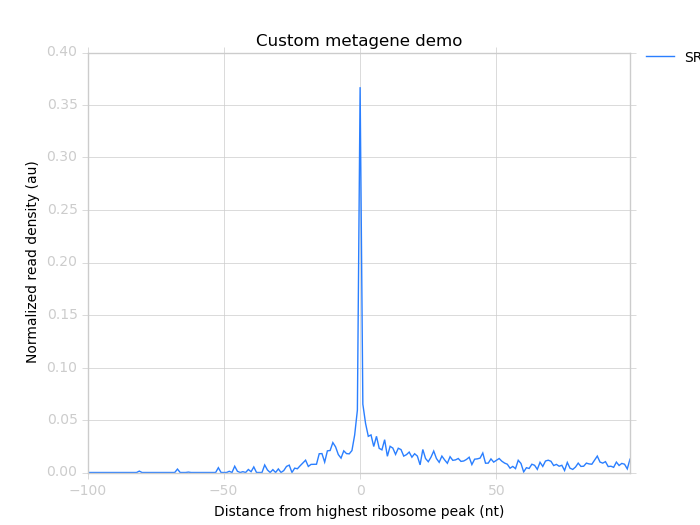
Metagene profile surrounding largest spike of ribosome density in coding region, excluding start and stop codon peaks.

---

See also

• Module documentation for metagene program for detailed description of command-line arguments and output files of the three subprograms