This tutorial illustrates how to measure read density over regions. As
an example, we look at gene expression (in raw read counts and RPKM)
using matched samples of RNA-seq and ribosome profiling data.
However, the analysis below can apply to any type of
high-throughput sequencing data (e.g. ClIP-seq, ChIP-seq, DMS-seq, et c).
This document aimed at beginners, and is broken into the following sections:
performing these analyses without using a mask file
to exclude repetitive genome seqence from analysis. In
practice, we would consider doing so. See
Excluding (masking) regions of the genome for a discussion of the
issues involved
not excluding start and stop codons from read density
measurements in ribosome profiling data. In practice,
we would do so, because start
and stop codon peaks, artificially
inflate estimates of steady-state translation.
Our first dataset is ribosome profiling, and we will map the ribosomal
P-site at 14 nucleotides from the 5’ end of each read (approximating [SGWM+12]).
To specify this, we use the arguments --fiveprime--offset14.
The data we want to count is in the file SRR609197_riboprofile_5hr_rep1.bam, which we pass
via --count_files. The genes we are interested in counting in this example
are on chromosome I, in the annotation file merlin_orfs.gtf. Finally,
we will tell the script to save the output in riboprofile.txt.
Putting this together, the script is run from the terminal as:
Gene expression – or, more broadly, read density over from any
high-throughput sequencing experiment over any genomic
region – can be calculated easily in an interactive Python
session.
In this example, we separately caclulate read density over:
Next, we tell the BAMGenomeArrays which mapping rule to use. We
will map the ribosome-protected footprints to their P-sites, which
we estimate as 14 nucleotides from the 5’ end of each read:
We will map the RNA-seq data along the entire length of each read alignment.
Each position in each alignment will be attributed \(1.0 / \ell\), where
\(\ell\) is the length of the read alignment.
CenterMapFactory() can do this for us:
Now, we need to create a place to hold our data. We’ll use dictionary of lists.
The call to copy.deepcopy() on the empty list is necessary to prevent all
of these dictionary keys from pointing to the same list, which is a weird side
effect of the order in which things are evaluated inside comprehensions:
>>> # we will count gene sub-regions in addition to entire genes>>> regions=("exon","5UTR","CDS","3UTR")>>> # we will calculate both total counts and RPKM>>> metrics=("counts","rpkm")>>> # create an empty list for each sample, region, and metric>>> my_data={"%s_%s_%s"%(SAMPLE,REGION,METRIC):copy.deepcopy([])\
>>> forSAMPLEinmy_datasets.keys()\
>>> forREGIONinregions\
>>> forMETRICinmetrics}>>> # add a list to our dictionary of lists to store transcript IDs>>> my_data["transcript_id"]=[]>>> # add additional lists to store information about each region>>> forregioninregions:>>> my_data["%s_chain"%region]=[]# SegmentChain representing region>>> my_data["%s_length"%region]=[]# Length of that SegmentChain, in nucleotides
Now that we have an empty dictionary of lists to hold our data, we’re ready to start
making measurements. We’ll use nested for loops to count expression in the 5’ UTR,
CDS, 3’UTR and total region (exon) of each transcript (note: this will run for a
while; you might want to get some coffee):
>>> fortranscriptinBED_Reader("merlin_orfs.bed",return_type=Transcript):>>>>>> # First, save ID of transcript we are evaluating>>> my_data["transcript_id"].append(transcript.get_name())>>> # Next, get transcript sub-regions, save them in a dict>>> # mapping region names to genomic regions (SegmentChains)>>> my_dict={"exon":transcript,>>> "5UTR":transcript.get_utr5(),>>> "CDS":transcript.get_cds(),>>> "3UTR":transcript.get_utr3()>>> }>>> # Iterate over these sub-regions for each transcript>>> forregion,subchaininmy_dict.items():>>> # Save the length for each sub-region>>> my_data["%s_length"%region].append(subchain.length)>>> my_data["%s_chain"%region].append(str(subchain))>>> # Iterate over each sample, getting the counts over each region>>> forsample_name,sample_datainmy_datasets.items():>>> # subchain.get_counts() fetches a list of counts at each position>>> # here we just want the sum>>> counts=sum(subchain.get_counts(sample_data))>>> rpkm=float(counts)/subchain.length*1000*1e6/sample_data.sum()>>> my_data["%s_%s_counts"%(sample_name,region)].append(counts)>>> my_data["%s_%s_rpkm"%(sample_name,region)].append(rpkm)
Finally, we can save the calculated values to a file. It is easiest to do this
by converting the dictionary of lists into a pandas.DataFrame:
>>> # convert to DataFrame, then save as tab-delimited text file>>> df=pd.DataFrame(my_data)>>> df.to_csv("gene_expression_demo.txt",sep="\t",index=False,header=True)
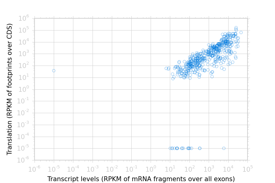
The text files may be re-loaded for further analysis, or plotted. For example,
to plot the RPKM measurements for translation (ribosome profiling)
and transcription (RNA-seq) against each other:
>>> my_figure=plt.figure()>>> plt.loglog()# log-scaling makes it easier>>> # make a copy of dataframe for plotting>>> # this is because 0-values cannot be plotted in log-space,>>> # so we set them to a pseudo value called `MIN_VAL`>>>>>> MIN_VAL=1>>> plot_df=copy.deepcopy(df)>>> df["RNA-seq_exon_rpkm"][df["RNA-seq_exon_rpkm"]==0]=MIN_VAL>>> df["ribosome_profiling_CDS_rpkm"][df["ribosome_profiling_CDS_rpkm"]==0]=MIN_VAL>>> # now, make a scatter plot>>> plt.scatter(plot_df["RNA-seq_exon_rpkm"],>>> plot_df["ribosome_profiling_CDS_rpkm"],>>> marker="o",alpha=0.5,facecolor="none",edgecolor="#007ADF")>>> plt.xlabel("Transcript levels (RPKM of mRNA fragments over all exons)")>>> plt.ylabel("Translation (RPKM of footprints over CDS)")>>> plt.show()
This produces the following plot:
Translation versus transcription levels for each gene
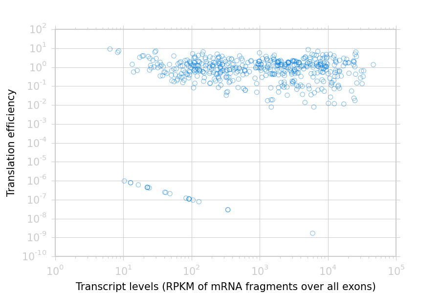
Translation efficiency is a measurement of how much protein is
made from a single mRNA. Translation efficiency thus reports
specifically on the translational control of gene expression.
There are many strategies for significance testing of differential gene expression
between multiple datasets, many of which (e.g. cufflinks and kallisto)
are specifically developed for RNA-seq These packages don’t require
plastid at all. For further information on them packages, see their
documentation.
For other experimental data types – e.g. ribosome profiling, DMS-seq,
ChIP-Seq, ClIP-Seq, et c – the assumptions made by many packages
specifically developed for RNA-seq analysis (e.g. even coverage across
transcripts) do not hold.
In contrast, the R package DESeq2 ([AH10, AMC+13, LHA14])
offer a generally applicable statistical approach that is appropriate to virtually
any count-based sequencing data.
Users are strongly encouraged to read the DESeq2 documentation
for a fuller discussion of DESeq’s statistical models with additional examples.
As input, DESeq2 takes two tables and an equation:
A table of uncorrected, unnormalizedcounts, in which:
each table row corresponds to a genomic region
each column corresponds to an experimental sample
the value in a each cell corresponds ot the number of counts
in the corresponding genomic region and sample
A sample design table
describing the properties of each sample (e.g. if any are technical or
biological replicates, or any treatments or conditions that differ between
samples)
A design equation, describing how
the samples or treatments relate to one another
From these, DESeq2 separately model intrinsic counting error (Poisson noise)
as well as additional inter-replicate error from biological or experimental
variability.
From these error models DESeq2 can detect significant differences in count
numbers between non-replicate samples, accounting for different sequencing depth
between samples.
The second table (in this example, rnaseq_sample_table.txt) is a description
of the experimental design. This can be created in any text editor and saved as a
tab-delimited text file. In this example, the we have two conditions, representing
timepoints at 5 and 24 hours post-infection:
With the count table, design table, and equation ready, everything can
be loaded into R:
># workflow modified from DESeq2 vignette at># https://bioconductor.org/packages/release/bioc/vignettes/DESeq2/inst/doc/DESeq2.pdf># import DESeq2>library("DESeq2")># load RNA seq data into a data.frame># first line of file are colum headers># "region" column specifies a list of row names>count_table<-read.delim("combined_counts.txt",>sep="\t",>header=TRUE,>row.names="region_name")># load experiment design table>sample_table<-read.delim("rnaseq_sample_table.txt",>sep="\t",>header=TRUE,>row.names="sample_name")># note, design parameter below tells DESeq2 that the 'condition' column># distinguishes replicates from non-replicates>dds<-DESeqDataSetFromMatrix(countData=count_table,>colData=sample_table,>design=~condition)># filter out rows with zero counts>dds<-dds[rowSums(counts(dds))>1,]># set baseline for comparison to 5 hour timepoint>dds$condition<-relevel(dds$condition,ref="5_hours")># run analysis>dds<-DESeq(dds)>res<-results(dds)># sort results ascending by adjusted p-value, column `padj`>resOrdered<-res[order(res$padj),]># export sorted data to text file for further analysis>write.table(as.data.frame(resOrdered),sep="\t",quote=FALSE,>file="5_vs_24hr_rnaseq_p_values.txt")># or, just select genes whose adjusted P-values meet significance level>res[res$padj<0.05,]># look at MA plot>plotMA(res,main="DESeq2")># see DESeq2 vignette for further information
Tests for differential translation efficiency can also be implemented in DESeq2.
The discussion below follows a reply from DESeq2 author Mike Love
(source here). We’ll
use the RNA-seq samples from above, plus some matched ribosome profiling.
Similarly, the design equation now needs an interaction term to alert
DESeq2 that we want to test whether the relationship between the two assays
to differ as a function of timepoint:
># load DESeq2>library("DESeq2")># load RNA seq data into a data.frame># first line of file are colum headers># "region" column specifies a list of row names>te_combined_data<-read.delim("te_combined_counts.txt",>sep="\t",>header=TRUE,>row.names="region_name")>>te_sample_table<-read.delim("te_sample_table.txt",>sep="\t",>header=TRUE,>row.names="sample_name")>># set up the experiment># note the interaction term in the design below:>dds<-DESeqDataSetFromMatrix(countData=te_combined_data,>colData=te_sample_table,>design=~assay+time+assay:time)># run the experiment>dds<-estimateSizeFactors(dds)>dds<-estimateDispersions(dds)>># likelihood ratio test on samples># compare model with and without interaction term>dds<-nbinomLRT(dds,>full=~assay+time+assay:time,>reduced=~assay+time)>>res<-DESeq(dds)>res<-results(dds)>summary(res)># Order results by P-value.># Column `padj` contains adjusted P-values for changes># in translation efficiency over time.>resOrdered<-res[order(res$padj),]>># export>write.table(as.data.frame(resOrdered),>sep="\t",quote=FALSE,>file="te_change_over_time.txt")># sneak a peak>head(resOrdered)
Website for DESeq2, as well as [AH10], [AMC+13] and
[LHA14] for discussions of statistical models for differential gene
expression, and examples on how to use DESeq/DESeq2 for various
experimental designs
Documentation for cs and counts_in_region for further discussion
of their algorithms